Hookes Law Experiment - Vaayu Puthran

Name : Vaayu Puthran a/l Shanmugaligam
Student ID : 29772974

What is Hooke's Law?

  When studying springs and elasticity, the 17ᵗʰ century physicist Robert Hooke noticed that the stress vs strain curve for many materials has a linear region. Within certain limits, the force required to stretch an elastic object such as a metal spring is directly proportional to the extension of the spring. This is known as Hooke's law and commonly written:         

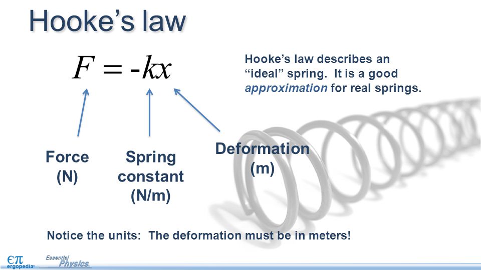             Source: https://www.google.com/urlsa=i&rct=j&q=&esrc=s&source=images&cd=&cad=rja&uact=8&ved=0ahUKEwiD1YnT9LvXAhUEpo8KHTm6BqcQjRwIBw&url=http%3A%2F%2Fslideplayer.com%2Fslide%2F3621957%2F&psig=AOvVaw3ez1Ggca3z8Iv3JiFVpSrx&ust=1510674849684468

$F$FFWhere F is the force, $x$

$Wherex$x is the length of extension/compression and $k$k is a constant of proportionality known as the spring constant which is usually given in $\backslash mathrm\{N/m\}$. .

What happens when a material is deformed?

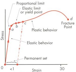
Source: https://www.google.com/url?sa=i&rct=j&q=&esrc=s&source=images&cd=&cad=rja&uact=8&ved=0ahUKEwjq-cixtL7XAhWLrY8KHfhZB9sQjRwIBw&url=https%3A%2F%2Fwww.leonghuat.com%2Farticles%2Fcivil%2520engineering.htm&psig=AOvVaw3eB-AsHlBdr9ZsPIv6n5XV&ust=1510760588744080

 During elastic deformation,When the stress is removed the material returns to the dimension it had before the load was applied. The deformation is reversible, non-permanent. However during plastic deformation, when a large stress is applied to a material. The stress is so large that when removed, the material does not spring back to its previous dimension. There is a permanent, irreversible deformation. The minimal value of the stress which produces plastic deformation is known as the elastic limit for the material.

Introduction

  A Hooke’s Law experiment that investigates the behaviour of three materials, giving the following set of results was carried out. The first two results, y1 and y2, are for two different elastic materials, which are both still in their linear regions. The results, z, describe the behaviour of a material which has gone past its elastic region (in the plastic region). x is the force applied (in Newtons) and y1, y2 and z are the deformation (in mm).

Source: https://marcelmayo.files.wordpress.com/2013/11/experiment.png

         Steps

1. The apparatus was assembled as shown above.
2. An initial reading was taken without any added mass to obtain a point of reference for the following readings.
3. A known force was applied to the spring which will cause it to displace.
4. The new length of the spring was measured and the procedure was repeated 9 times increasing the amount of force applied each time.
5. The experiment was repeated for material y1, y2 and z.

 The results were analysed and what is happening physically to the materials investigated will be discussed. The differences between the three graphs, discuss and the possible explanations for any errors that might be seen from the graphs would also be discussed in this post.

Calculations

The values of material x(N), y1(mm), y2(mm) and z(mm) were given as follow :

x   = 1.00, 2.00, 3.00, 4.00, 5.00, 6.00, 7.00, 8.00, 9.00

y₁ = 3.00, 4.50, 6.00, 7.50, 9.00, 10.50, 13.00, 14.00, 15.00

A graph of y versus x was drawn. The values of a and b were found from the given formula :

y1 = ax + b

The values of y2 are given by :

y2 = (a + 0.5x) + c  ,  where c = 0.2

The values of z are given by :

z = x³ + b

 The values of a and b was found in the gradient and the y-intercept of the equation 
y1 = ax + b respectively. The values of y2 and z are found using Microsoft Office Excel by inserting the following formula under the value's column as shown in Figure 1 :

FIGURE 1

where the value of c is given as 0.2, a is 1.5583333333 and b is 1.375

Tabulation of data

The values of a and b was found after the graph of y versus x was drawn on Excel. All the values are then tabulated into a set of data :

FIGURE 2

x (N)	y1 (mm)	y2 (mm)	z (mm)
1.00	3.00	2.2583	2.375
2.00	4.50	4.3166	9.375
3.00	6.00	6.3749	28.375
4.00	7.50	8.4332	65.375
5.00	9.00	10.4915	126.375
6.00	10.50	12.5498	217.375
7.00	13.00	14.6081	344.375
8.00	14.00	16.6664	513.375

where x is the force applied (N), y1 , y2 and z are deformations (mm)

The graph of y2 was drawn on the same graph as y1. The intercepting point between both of the graphs were found using simultaneous equations in Excel. Figure 3 shows the graph of y1 versus x and the graph of y2 versus x. Figure 4 shows the graph of z versus x.

FIGURE 3

FIGURE 4

Based on Figure 3, the intersection point of y1 and y2 is (2.35,5.037). The intersection points can be found using simultaneous equations. The methods are shown below :

The intersection points can be found using simultaneous equations in Microsoft Office Excel.

The intersection points can also be found by solving the simultaneous equations manually.

Discussion

  Materials y1 and y2 are in their elastic region of deformation. This can be said as a linear graph can be obtained for both of the graphs in the figure. Therefore a directly proportional relationship between the displacement of the material,y and the force applied,x can be obtained. Thus, when the force is applied it is displaced and returns to it's original position when the force is released.

 Material z is in it's plastic region of deformation. This can be seen from the exponential graph that was obtained by plotting the values of z. Therefore, when force is applied to the material, it cannot return to it's original position as it has gone past it's elastic region.

  From Hooke's Law, F = kx. The graph of y(mm) versus x(N) is likely similar :

1/k = y/x

 Therefore we can conclude that the gradient of the graphs are equal to one over the stiffness of the spring.

m = 1/k

 Thus, the steeper graph has lower stiffness compared to the other graphs. According to Figure 3, the graph of y2 is steeper compared to y1. Thus, material y2 has lower stiffness compared to material y1. The graph of y2 is also steeper than the graph of y1 because material y2 is more elastic than material y1. When the graph of y2 is steeper than the graph of y1, material y2 requires less force to produces a larger elastic displacement compared to material y1.

 When the graphs in Figure 4 is brought to a comparison with Figure 3, the displacement for material z is higher with force compared to material y1 and y2. This is because there is a restoring force that resists the force applied on materials y1 and y2 while the force applied on material z permanently displaces material z.

 The possible error that may have occurred to cause inaccurate values to be obtained is the error made when taking the measurement of the displacement of the materials. This parallax error may greatly affect the outcome of the experiment. Besides that, when solving the simultaneous equations, the values of y and x as the point of intersection between graphs y1 and y2 were rounded off to two decimal places.The systematic error 

 Therefore, the outcomes and the values obtained from materials from different regions of deformation confirms that Hooke's Law is true. The materials y1 and y2 would obey Hooke's Law until it have exceeded it's elastic limit.

Referencing list

1) Anon, n.d. What is Hooke's Law? (article). [online] Khan Academy. Available at: <https://www.khanacademy.org/science/physics/work-and-energy/hookes-law/a/what-is-hookes-law>

2) Trivett, F., 2017. Hooke's law This lesson introduces forces from springs and Hooke's law: F = −kx. The presentation begins by describing types of springs and distinguishing. [online] SlidePlayer. Available at: <http://slideplayer.com/slide/3621

3) Anon, n.d. [online] Importance of Yield Strength & Plastic Deformation to Civil Engineers. Available at: <https://www.leonghuat.com/articles/civil engineering.htm>

4) Marcelmayo, n.d. marcelmayo. [online] marcelmayo. Available at: <https://marcelmayo.wordpress.c